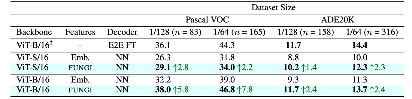
No Train, all Gain: Self-Supervised Gradients Improve Deep Frozen Representations

Our method is composed of two main parts: the extraction of unsupervised gradients from a pretrained backbone and the construction of FUNGI features. Figure 1 illustrates the gradients extraction procedure, including the downsampling step using random projections, while Figure 2 shows how FUNGI features are built.

Figure 1: Overview of our method with a SimCLR loss. Given a pretrained backbone \(f\) and a randomly initialized projection head \(h\), we first patchify an image, obtain a latent representation of the patches (1), calculate the SimCLR loss by maximizing the pairwise cosine similarity of patches belonging to the same image, and minimizing their similarity to a fixed negatives batch and backpropagate (2), extract the per-sample gradients (3) and finally project the gradients to the same dimensionality as the embeddings (4).

FUNGI features are constructed by concatenating one or more gradients to the model embeddings after \(L_2\)-normalizing each component independently to ensure they are considered equally. If we define \(g_{\beta_i}(x)\) as the gradients for the \(i\)-th objective, \(f(x)\) to be the model embeddings and \(z' = z/||z||_2\) as the \(L_2\) normalization operator, we can construct FUNGI features as follows:

$$\phi(x) = \mathrm{\texttt{cat}} \left[ g_{\beta_1}'(x), g_{\beta_2}'(x), ..., f'(x) \right].$$ Figure 2 illustrates the construction of FUNGI features and their nearest-neighbor index graphically.

Figure 2: FUNGI features: given a pretrained backbone \(f_{\theta^*}\) and its embeddings, we apply a family of SSL losses, extract their gradients, and project and concatenate them. These new features are used to build a \(k\)-nearest neighbor index, which can be used for classification or retrieval.

We show that FUNGI features yield non-trivial performance improvements across several backbones and datasets. Figure 3 shows that both in a full dataset and in a few shot (using 5 examples per class) setups, FUNGI features improve the classification accuracy, even for strong backbones such as DINOv2. Table 1 shows the per-dataset performance improvements for FUNGI features constructed using KL, DINO, and SimCLR gradients for two supervised ViT-B/16 backbones pretrained using IN1K and IN21K. Table 2 shows that combining multiple gradients translates to improved downstream performance.

Figure 3: FUNGI works across backbones. Top-1 accuracy in \(k\)-nearest neighbor classification of embeddings versus FUNGI features on various ViT backbones, both for full dataset and few shot setups, averaged over 11 datasets. For the FUNGI features, we chose the best-performing combination across datasets. "AR" indicates backbones trained with the AugReg strategy.

Table 1: FUNGI features are better on several datasets. Accuracy of embeddings and FUNGI features in \(k\)-nearest neighbor classification over 11 datasets, for two AugReg ViT-B/16 models from timm pretrained on IN1K and IN21K respectively.

Table 2: Performance improves as more gradients are used. Average accuracy over 11 datasets in image classification using \(k\)-nearest neighbor with embeddings and FUNGI features, built by incrementally adding gradients. We show results for 7 backbones in the full dataset and few shot setups. "K", "D" and "S" stand for KL, DINO and SimCLR, respectively.

While our experiments focus on vision tasks, we show that, in principle, FUNGI features can improve text and audio encoders' \(k\)-nearest neighbor classification abilities, using 5 text and 2 audio datasets and 3 transformer backbones. We extract gradients using the \(\mathcal{L}_\text{KL}\) and \(\mathcal{L}_\text{SimCLR}\) losses, using the same formulation as in vision tasks with minor modifications. The \(\mathcal{L}_\text{SimCLR}\) views are obtained by deleting random words with a 10% probability or by applying additive noise to input samples for text and audio inputs, respectively.

For both modalities we are able to obtain significant accuracy improvements, up to 16.1% for text and 4.2% for audio. We expect that language or audio-specific self-supervised losses would yield even more predictive gradients.

Table 3: FUNGI features are useful for the text modality. Top-1 accuracy in \(k\)-nearest neighbor text classification on 5 datasets, for the full dataset and few shot (using 5 shots) setups, using BERT and T5 backbones. "K" and "S" stand for KL and SimCLR, respectively.

Table 4: FUNGI works for audio. Top-1 accuracies in \(k\)-nearest neighbor audio classification of embeddings and FUNGI features obtained from a SSAST backbone on 2 datasets, for the full dataset and few shot (using 5 shots) setups. "K" and "S" stand for KL and SimCLR, respectively.

We evaluate FUNGI features in the task of in-context scene understanding introduced by Balazevic et al. In particular, we perform retrieval-based semantic segmentation on PASCAL VOC 2012 and ADE20K. We oobtain the gradients used to build FUNGI features via a SimCLR-style loss that minimizes the distances between patch embeddings belonging to the same image and maximizes the distance to nearest-neighbors of those patches retrieved from a support index. Please refer to our paper for further details about the methodology and experimental setup.

We show that, compared to the raw DINO patch embeddings, our FUNGI features are up to 17% better and that in a few-shot experiment, we also outperform end-to-end finetuning of DINO for semantic segmentation on Pascal VOC. Moreover, the DINO ViT-B/16 model, when enhanced with our FUNGI approach, achieves competitive results against the current state-of-the-art HummingBird model, with a difference of only 3.5% on Pascal VOC and 3.1% on ADE20K, without any training.

We summarize our results in Table 5 and 6, the first showing the results for the full-dataset evaluation and the second for the data-efficient one. We also provide some qualitative results in Figure 4, showing that our method produces sharper and more complete segmentation masks.

Table 5: FUNGI features improve in-context semantic segmentation. mIoU for retrieval-based semantic segmentation on Pascal VOC 2012 and ADE20K, comparing a DINO baseline against FUNGI features and the self-supervised HummingBird model. Results from Balazevic et al. are marked with \(\ddagger\). We resize each image to \(512 \times 512\) and extract \(32^2 = 1024\) patch features.

Table 6: Data-efficient semantic segmentation. mIoU scores for data-efficient retrieval-based semantic segmentation on Pascal VOC 2012 and ADE20K, using DINO backbones and their FUNGI features and embeddings. We also compare FUNGI to end-to-end fine-tuning and find our method to perform best for VOC. Results from Balazevic et al. are marked with \(\ddagger\).

Figure 4: FUNGI produces sharper and more complete segmentation masks. Segmentation masks produced via nearest neighbor retrieval using DINO features (left), FUNGI (center), and the ground truth (right). Both methods use a memory bank of \(1024 \times 10^4\) patches.

We evaluate the performance of FUNGI features in image retrieval using the revisited Oxford and Paris landmarks datasets. We report the mean average precision (mAP) for both the medium (M) and hard (H) splits, using the evaluation protocol of DINO.

The results are displayed in Table 7 and show that FUNGI improve the retrieval abilities of all backbones, except DINOv2. Our method is particularly effective for CLIP: on Paris (H), we improve by 12.4% and 7.2% for CLIP and EVA-CLIP, respectively.